Understanding Computational Graphs
Before we continue with our cat problem I would to use the lesson to introduce a visualization tool known as computation graphs.
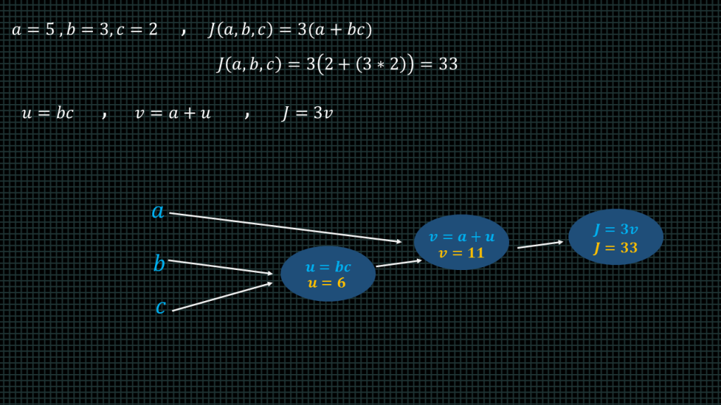
Lets say we have a function j of a b c equals 3 into brackets a plus bc.
Lets say a = 5, b=3, and c =2.
When we insert this into our function the result is 33.
Now lets break the function down into smaller funtions
We are going to represent the b times c part of the function with a variable u, and then create a new variable v such that v equals a plus u. f we substitute these new variables into our function J becomes equal to 3v.
We can represent this in a computational graph by creating 3 nodes, one u, one for v and one for “J”.
“B” mulitiplied by c gives us u which is equal to 6.
“A + u” gives us “v” which is equal to 11.
3 multiplied by “v” gives us J which is equal to 33.
This is the computation graph of our function. Now lets see how to compute the derivatives of our function using this computation graph.
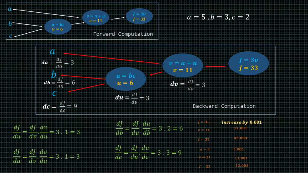
Lets start by computing the derivative of with respect of v. This is written as “dj/dv”. This simple means that if we change the value of “v” how much will the value of J change.
And the answer is 3. We know “j” is always 3 times the value of “v” so whatever increment we make to “v” that increment is going to be multiplied by 3 to get the corresponding “j” increment.
As we can see in this simple example here when we increment “v” by 0.001, “j” is incremented by 0.003.
By computing the derivative of “v” we have essentially done one step of backpropagation.
Backpropagation involves computing the derivative of the final output variable with respect to the intermediary variables.
Now, lets try to compute the derivative of the final variable “J” with respect to the variable “a”.
In other words, lets see how much the final variable “J” will increase if we increase the variable “a”.
“A” is 5 if we increase “a” by 0.001, “a” becomes 5.001.
“v” equals “a + u”, “u” is 6 so the new “v” value becomes 6+5.001 , this will give us v = 11.001, “J” is 3 times v, 3.
3 times 11.001 is equal to 33.003. As we can see we increased “a” by 0.001 and “j” got increased by 0.003. This shows that the derivative of “J” with respect o “a” is 3.
Mathematically, what we essentially did is find the derivative of “v” with respect to “a” and then multiply the result by the derivative “j” with respect to “v”.
This is because in order to find how much “a” will increase if we increase “a”. We have to find how much “v” will increase if we increase “a” and then find out how much “j” will increase if we increase v. This because in our computation graph. “a” connects to “v” and “v” connects to “j”.
This also proves the chain rule of derivatives we mentioned in a previous lesson.
Dj/da = dj/dv times dv/da.
Now lets see how to solve for “dJ/db”. Meaning when we increase the value of the variable b how much will the final variable increase.
To do that, we have to first find “du/db” . Meaning when we increase the variable b how much will the variable “u” increase. Remember “u” equals “b” multiplied by “c”. We said the variable “c” equals 2 .The equation “u” is effectively “u = 2b”, if we replace “c” here by its value “2” then indeed “u” becomes equal to 2 multiplied by “b”. This means that whatever increase we make to the variable “b” it going to be multiplied by 2. Such that when we increase the current value of “b” which is equal 3 to 3.001, “u” becomes 6.002, because we will derive “u” by computing 2 multiplied by 3.001.
So then the “du/db” is equal to 2. This means when we increase the variable “b” by a particular amount. The variable “u” is going to be increased by twice that amount.
Now that we now the derivative of “u” with respect to “b” is 2 we simply need to find the derivative of “j” with respect to “u”. Wait a minute, we have already computed that. We have already computed how much the final variable “j” will increase when we increase the variable “u” .The answer was 3.
By multiplying “dj/du” by “du/db” we get “dj/db”. This is the chain rule at work again.
We apply the same method to derive “dj/dc”.
Lets see you we can apply what we have learnt about computation graphs to our logistic regression example.
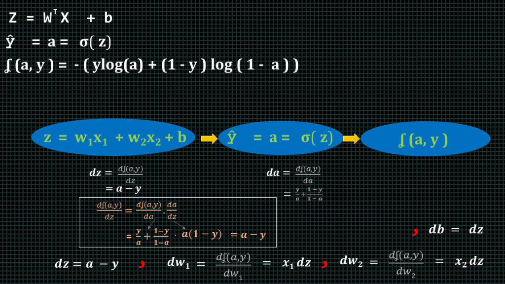
We said we compute “z” by “w” transpose “x” plus “b”
We then pass “z” through our activation function to derive “yhat” or “a”.
We also defined our loss function to be this equation.
We can represent this in a computation graph like this.
We take “w”,”x” and “b” to compute “z”.
We take “z” to compute “yhat” which we also call “a” over here.
After computing “a” we apply our loss function. Remember “a” is the same as “yhat” which is our predicted value. “y” is the expected value.
So our is to compute the derives with respect to the loss.
We start by computing the derivative of the loss with respect to the variable “a”.
When we take the loss equation up here and we compute the derivative this is the answer we get.
When we compute the derivative of the loss with respect to “z” we get the answer “a-y” When we compute further we will find that the derivative with respect to “w1” which we have named here “dw1” is equal to “x1dz”. Similarly the derivative with respect to “w2” which is named here as “dw2” is “x2dz”. This essentially gives us how much we need to change the “w” values in order to minimize to loss and finally, “db” is equal to “dz”
Updating parameters
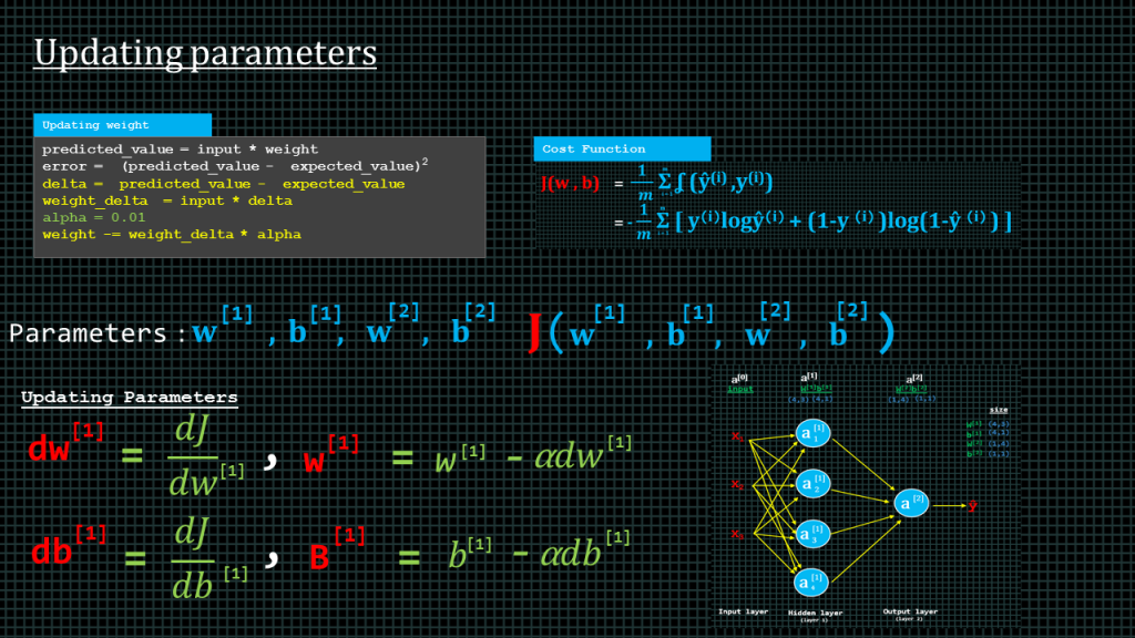
Earlier on in the course we saw how to update the weight parameters using a very simple method.
Our error or loss function in that lesson was predicted value minus expected value squared.
We introduced delta which we called the pure error and we expressed it by simply: predicted value minus expected value without the squared.
We went on to compute the weight delta by multiplying the delta by the input.
And we said in order to prevent over scaling we had to introduce a new constant known as the learning rate or alpha.
We then updated the weight by multiplying the weight delta by alpha and then subtract the answer from the current weight value. As we can see over here. This what we showed before to demonstrate the concept of learning and updating the weight based on what is learned.
Lets see how that same concept can be applied here to our cats or no cat simple logistic regression example.
Our cost function is expressed by this equation as we saw some lesson ago.
Our neural network has four parameters. W1 and b1 are the weight and biases of layer one. What these mean is, these are the weights and biases which are multiplied and added to the input to derive the result “z subscript 1 “
“z subscript 2”, “z subscript 3”, and “z subscript 4” which are ultimately passed through our activation function to obtain “a subscript 1”, “a subscript 2”, “a subscript 3” and “a subscript 4”.
“ W superscript 1”, and “ b superscript 1” are therefore known as parameters of layer one because they give us the results of “layer1”.
We also have “ w superscript 2” and “b superscript 2” these parameters take the result of layer 1 and transform it to give us the result of layer 2 using the same method I just described.
So in our two layer neural network we have 4 parameters. 2 for layer 1 and 2 for layer 2. Remember as I mentioned earlier when counting the layers of a neural network we don’t count the input layer.
So, back to the cost function.
We have to find the cost with respect to these for parameters so that we can reduce the error between what they currently are and what they need to be in order to give us a predicted value which is as close to the expected value as possible.
We will update w1 by computing dj dw1 and then multiplying the result by our learning rate alpha and then subtracting the result from the current w1 to get the new w1
We will update b1 by computing dj db1 and then multiplying the result by our learning rate alpha and then subtracting the result from the current b1 to get the b1. Like we can see over here.
We do the same thing to update w2 and b2.
This is how we shall update the parameters.
Vectorization
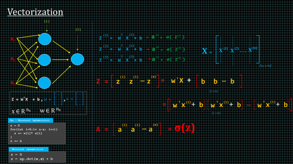
The goal of vectorization is to avoid explicit “for-loops”.
Let me explain. We know to derive “z” we compute “w” transpose “x” plus “b”. Let’s say we have stored our “w” values in a 1-dimensional array or column vector and our “x” values also in its 1-dimensional array or column vector. To compute this we will use are for loop to do something like this.
This single look shall be used to compute a single “z” value. We doing this computing element by element. This takes extremely long to compute.
In programming languages such as python, there are libraries that can be used to perform this kind of computation over 100 times faster. The “numpy” library can be used to do this. In “numpy” we can compute the entire “z” vector without doing it element by element by simply doing “np.dot(w,x)+b”.
Apart from allowing us to compute the entire vector without “for-loops” the numpy library is also implemented using the “SIMD” instructions of the processor which makes it optimized for computations such as this one. “SIMD” stands for single-instruction-multiple-data. This allows data to processed in parallel manner with fewer processor cycles.
Let’s say we have some training examples. To compute the prediction of the first training example we compute for “z” and then we use “z” to find “a”. Note that over here I am using actual brackets rather than square brackets, this is to indicate that they are training example numbers not layer numbers.
We can compute the predictions for the second and the third by doing the same. If we have 10,000 training examples we will need to do this 10,000 times.
We can compute this faster by applying vectorization.
Remember, each example is a column vector, in other words, 1 -dimensional array. The length of each example is equal to the number of features which we call “n” subscript “x”.
We can put all our training example together in a single matrix. We call this matrix capital “X”. the first column of the matrix represents the first training example, the second column represents the second training example, all the way to the last training example which we have denoted as “m”. Therefore the size of the matrix “n” subscript “x” by “m”.
We can also put all the biases “b” together in a single row vector like this.
Having done this we can compute the “z” for all the training examples, all at once by perform “w” transpose capital “X” which contains all our training examples. Plus row vector “b” which contains the baise for all the training examples.
This will give a row vector capital “Z” which contains the z results of all the training examples. If we take capital “Z” and apply our activation function we get capital “A” which is a row vector containing the “a” values of all training examples.
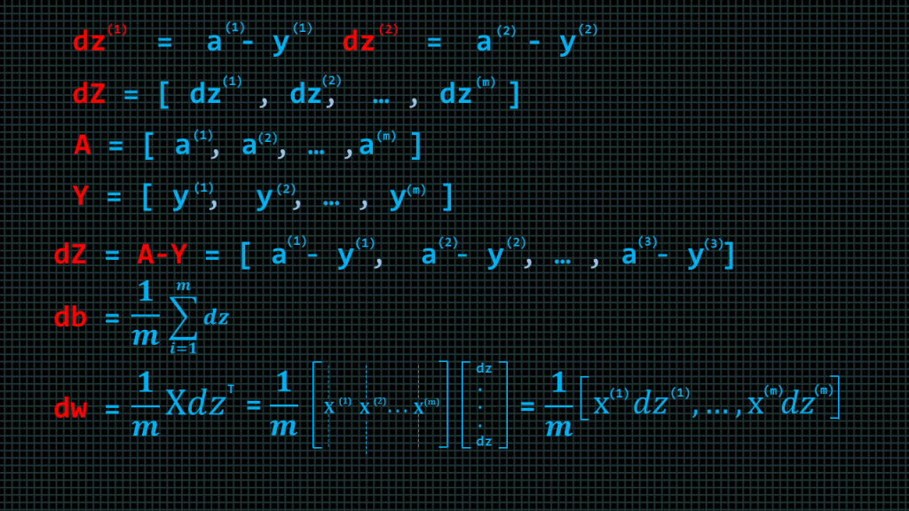
Earlier we deduced that to find the loss with respect to ”z” we compute “a-y”, which we call “dz”. So the “dz” of training example 1 is written here as “dz” superscript1 and “dz” of training example 2 is written as “dz” superscript 2. We can put all the “dz” together in a row vector which we call “d” capital “Z”. We have all the “a’s” in a row vector which we call capital “A”. Similarly, we can put all the “y’s” in a row vector which we call capital “Y”. We can compute “dz” of all the training examples by simply doing “d” capital “Z” equals capital “A” minus capital “Y”.
“db” of the all the training examples can be computed by finding the average of “dz”, and finally, “dw” of all the training examples can be computed by finding the average of capital “X” “dz” transpose. We shall see how to compute all of this in code.
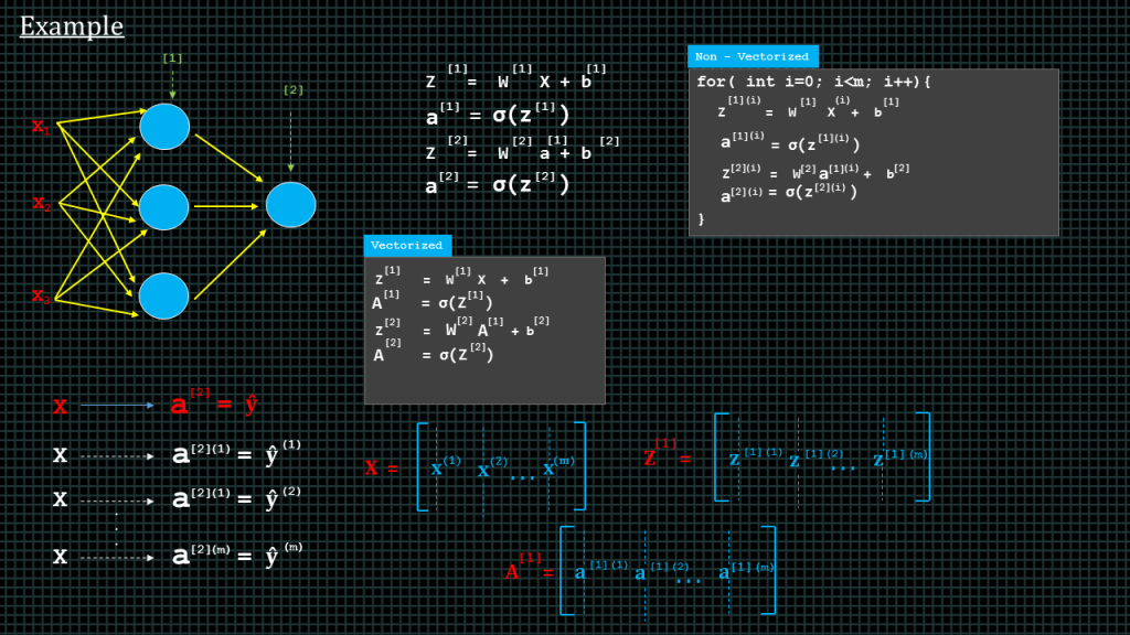
Lets say we have a two layer neural network such as this one over here.
As we you are by now familiar with, we to find “a” superscript 2 which is equal to “yhat” we first find “z” superscript 1 and then use that to find “a” 1 and then use “a” superscript 1 to find “z” superscript 2 and then finally use “z” superscript 2 to find “a” superscript 2.
This is for just one training example.
To execute this in code for “m” training examples, this is how we shall implement it in code. We shall essentially perform these steps “m” times
Just to remind you again x1,x2,x3, does not mean training examples. These are features of each training example, in other words each training example has 3 inputs.
So training example1 will produce yhat 1, which is the same as “a” superscript square bracket2, bracket 1. The square bracket indicates the number and the normal bracket indicates the training example number.
In same way the training example 2 will produce yhat 2 nd training example 3 will produce yhat3.
So to “vectorize” this, we take all our training example and put them in a single matrix called capital “X”.
We shall also keep all our “z” superscript1 results in a matrix like, the “a” superscript1 result in a matrix like this, as well the “z” superscript2 and the “a” superscript 2 in their own matrix.
We can then simply take these “vectorized” matrices and compute “a” superscript2, which is the same as yhat like this.
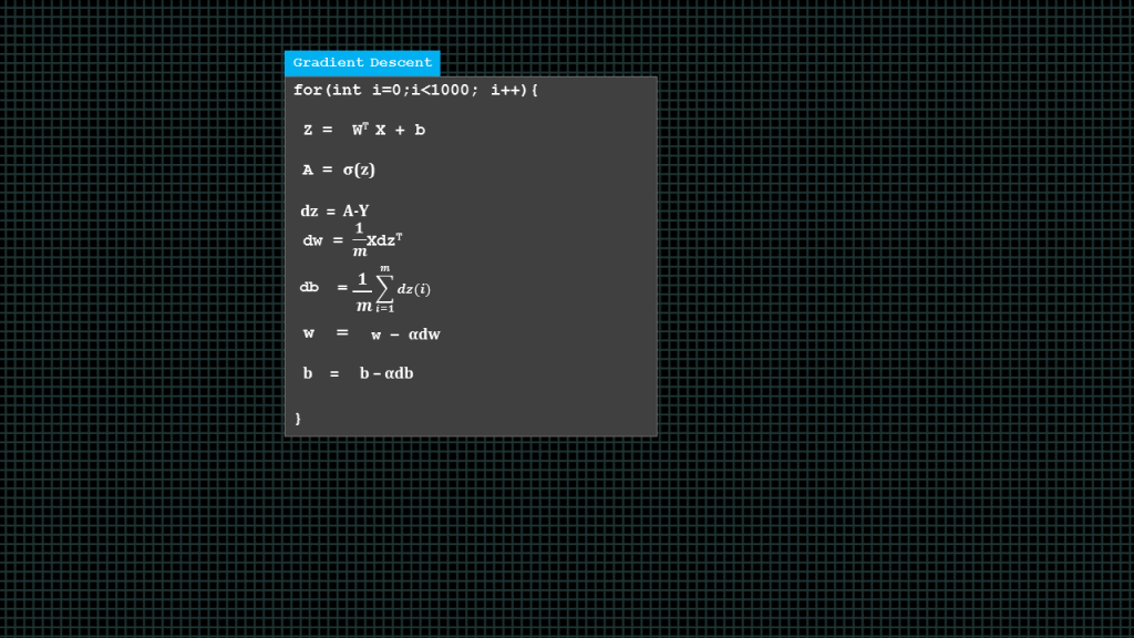
In summary this what a complete gradient descent function looks like.
We compute all “z” values, and then all “A” values,then we find “dz”, “dw” and “db” once we have found these derivatives we go ahead to update our weights and biases.
Over here it is in a “for-loop” because we want to perform multiple iterations of gradient descent. I’m just using 1000 here as an example. Now, lets summarize what we have learnt so far about forward propagation and back propagation
ForwardProp and Backprop Summary
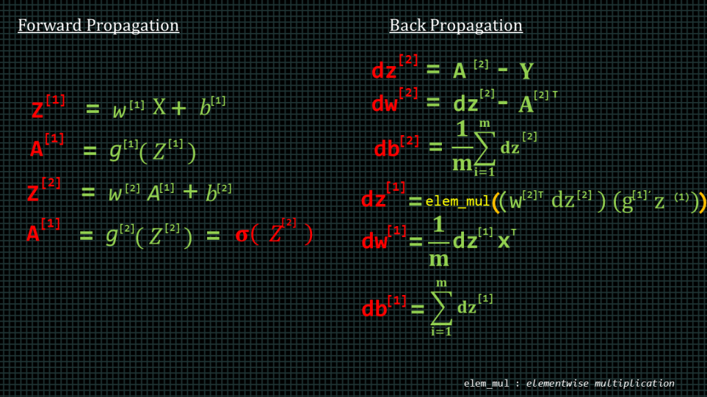
These are the steps to compute the forward progapation of our neural network. Over here we are using the function “g” to denote an activation function.
Backpropagation involves computing the derivative with respect to our parameters so that we can use the derivatives to update our parameters.
Parameters Initialization
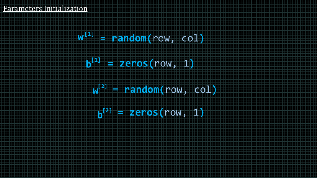
When we create the arrays to hold our parameters we have to initialize them. We have to initialize the weight matrices or arrays with random values, and the baize matrices or arrays with zeroes, as we can see over here. Presumably the pseudo function “random(row,col)” which generate a matrix of “row” number of rows and “col” number of columns and fill the matrix with random numbers.
Broadcasting
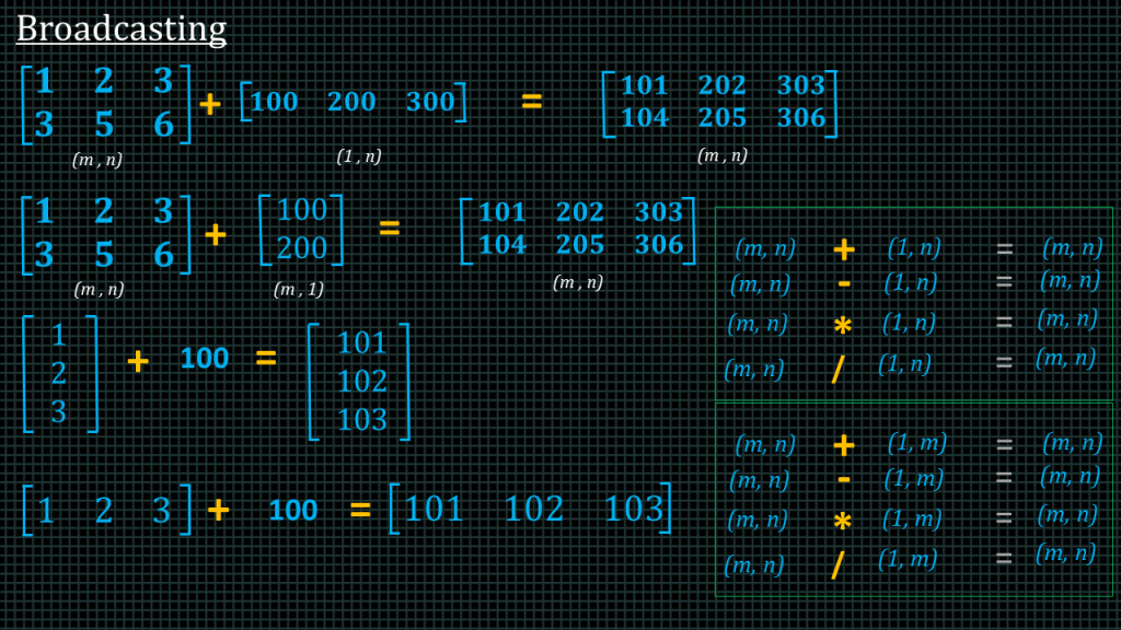
The term broadcasting describes a programming language treats arrays with different shapes during arithmetic operations. Generally,the smaller array is “broadcast” across the larger array so that they have compatible shapes. Lets see an example.
Lets say we have this 2 by 3 matrix and we add this 1 by 3 matrix. The result is a 2 by 3 matrix like this. We essentially add the row content of the smaller matrix onto each row of the larger matrix.
Lets say we have this 2 by 3 matrix again and this time we add this 2 by 1 matrix. The result produced is a 2 by 3 matrix. This time we take the column content of the smaller matrix and add it to each column of the larger matrix.
If we have a matrix or vector and we add scalar value, the value is add to each member of the matrix.
This works for all the basic arithmetic operations, meaning addition, subtraction, division and multiplication.
Add Comment