Common notations.
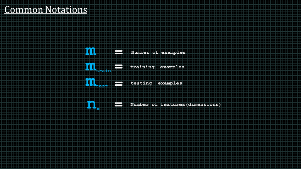
In machine learning, training examples are are often represented by the letter “m”.
We often break our training examples into 2 sets. Training set and test set.
We training set it often denoted by “m” subscript train
And the test set denoted by “m” subscript test.
We denote the number of features by n. You can think of number of features as number of inputs.
In our previous examples the our nueral network had two features. Hours of rest and hours of workout.
When we working with image recognition the number of features becomes the number of pixels in the image because we will have to feed each pixel into the nueral network.
Cat or not cat ?
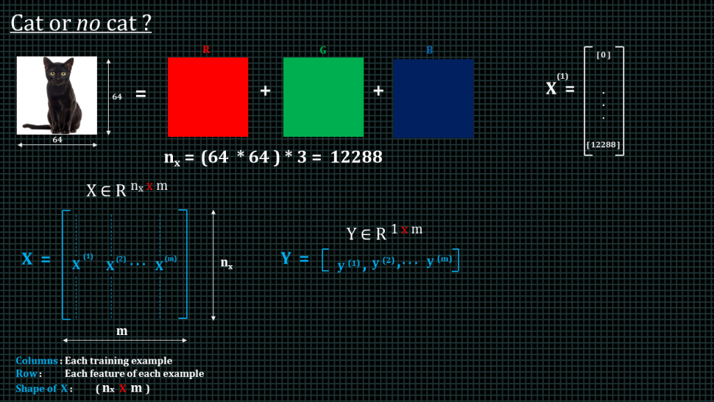
Lets say we want to design a neural network for a binary classification problem. Lets we want our neural network to take a 64×64 image and tell us if the image has a cat or not.
To store an image our computer
stores three separate matrices corresponding to the red, green, and
blue color channels of this image. So if our input image is
64 pixels by 64 pixels, then we would have 3 64 by 64 matrices corresponding to the red, green and blue
pixel intensity values for our images.
To turn these pixel intensity values into a feature vector, what we need unroll all of the pixel
values into an input feature vector x, like this. We simply need to take the red matrix which is a 2D array and convert it to a vector meaning a 1D array. We do that by listing the pixel values vertically. We take the first row, we write the first value, and then we write the second value below the first value, and then we write the third value below the second value.Once we are done with the first row we continue by listing the value of the second in the same vector, we put the second row values under that of the first row. We continue doing this until we added all the rows of the red channel. Once that is done we move on to the green channel and list the pixel values of the channel under the pixel values of the red channel in the same vector.
Once this is done we move on to the blue channel and do the same thing.
We will end up with 12,288 features.
So each training example will have 12,288 features.
The training examples are put together in matrix denoted here as capital “X”. Capital X then becomes our input matrix representing all training examples and the features.
Each column in input matrix capital X represents a single training example.
The first row of input matrix capital X represents the first feature of the training examples. I should remind you that whenever I say features should simply think of inputs.
Input matrix X shall be processed by the neural network column by column. Remember again that column represents each training example.
Capital X belongs to real numbers and the dimension of capital X is number of features by number of examples.
The training labels shall be kept in a vector capital Y
Whereby y1 is the answer to the question is x1 are cat or not. And y2 is the answer the answer to the question is x2 are cat or not and so on and so forth.
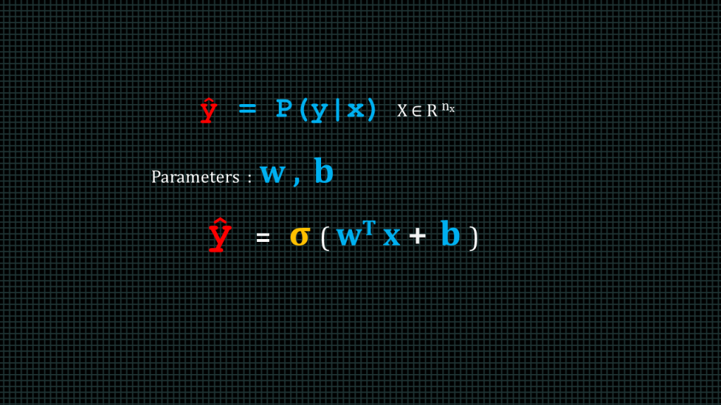
Yhat is the value that we predicted whereas y is the value we expected. We can say Yhat the is the probably of y given that we know x
Our neural network often have two parameters. W, and b.
We shall talk about hyperparameters later on in this course.
W is known as the weight matrix and b is known as the bia.
We compute yhat by performing a dot product operation between the transpose of the weight matrix and the input matrix, add the bias b and then apply an activation function to the results.
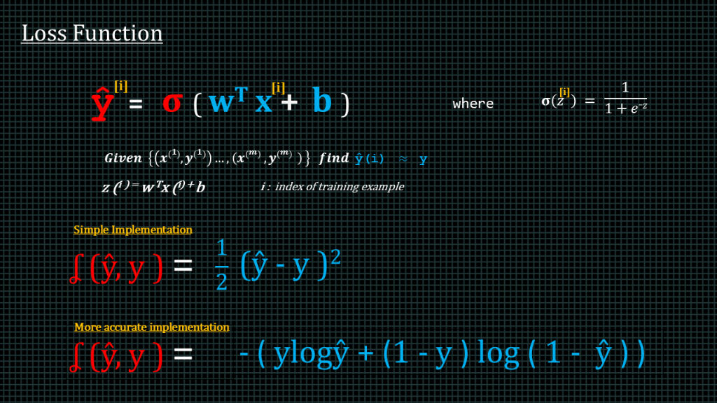
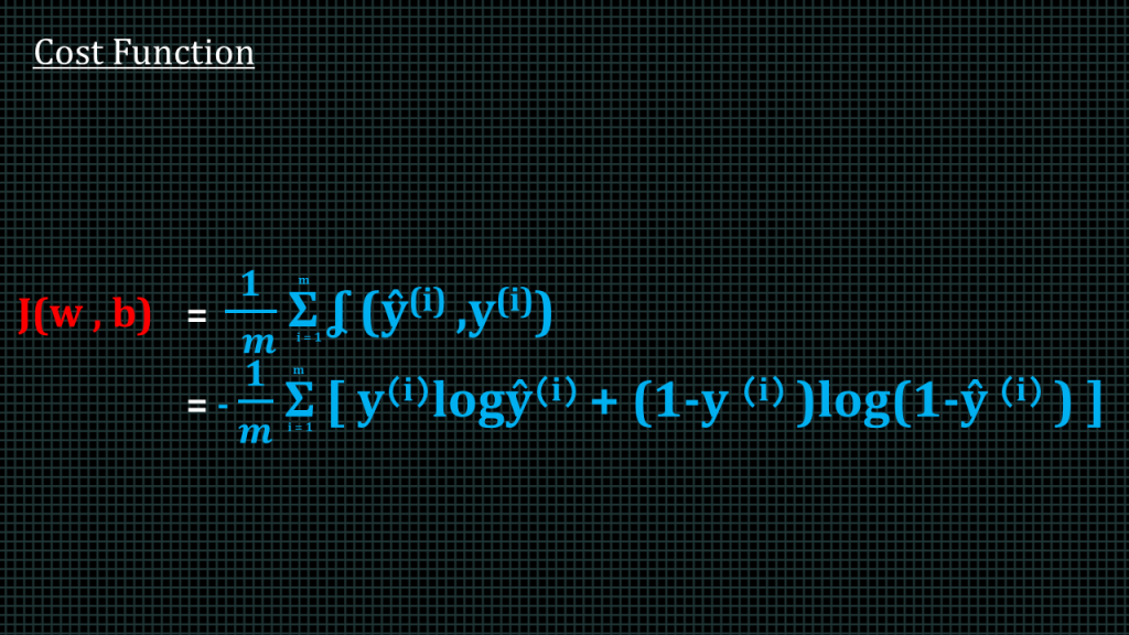
Now lets take a look at our logistic regression loss function. The loss function is simply the function for calculating error.
The simplified loss function we saw in previous lesson looked like this. Predicted value – expected values, we square the difference and then multiply by half.
A more accurate loss function for logistic regression is this.
Negative into bracket ylogyhat +1-y log1-yhat.
Next slide :
Remember the loss function is applied to just a single training example. The cost function is the cost of all the parameters. In other words the cost function is the average of all the loss functions. This is what the cost function looks like. We are adding up all the loss functions and the dividing the result by the number of training examples.
This is the cost function we shall train our neural network with when we go to code.
This brings us to the end of this lesson. I shall see you in the next lesson.
Internals of a 2-layer Neural Network
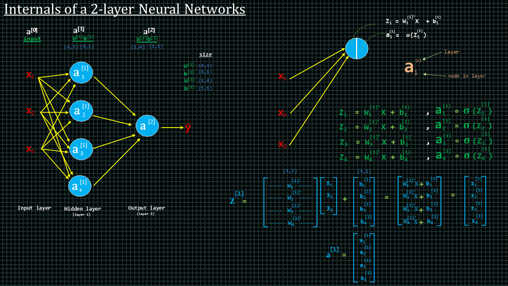
Lets say we have a 2 layer neural network
Like this. We don’t often include the input layer when we talk about the layers of a neural network. Hence a two layer neural network will look like this. The input layer is always denoted as a0 the next layer is denoted as a1 and the one after that as a2.
The hidden layer a1 has 4 units, The superscript represents the layer number and the subscript represents the unit number.
Let see how to compute unit a subscript 1 superscript 1
To compute this we begin by computing z subscript 1.
Z subscript 1 is computed by weight subscript 1 transpose x + b suscript1 superscript 1. Remember we use subscript to denote the unit number as superscript to denote the layer number.
Once we have found z subscript 1 we apply our activation function to it to get a subscript 1 superscript 1. This is how we find the output of the first unit.
We find the outputs of the second, third and fourth units using the same method but we have to use their respective weights and baises. Like shown in these equations
To compute z superscript 1 which means the z outputs of the entire layer number one. We put all the weights together in matrix and, all the inputs in a vector and then all the biases in a vector and perform w transpose x plus b on the matrix and vectors. The results will look like what we see over here. We end up with a vector containing the z results of the of all the units in layer 1. By applying our activation function to this result we get a new vector containing all the a results of layer 1.
Also take note of the dimensions of parameters. The dimension of the weight matrix is 4 by 3. 4 rows, 3 columns. 4 rows because layer 1 has 4 units and 3 columns because we have 3 inputs entering each unit. We shall spend more time talking about ways to fully understand the dimensions later.
Activation Functions
Activation functions introduce non-linear properties to our Network. Their main purpose is to convert an input signal of a unit or node in our neural network to an output signal. That output signal is then used as an input in the next layer.
We do the sum of products of inputs(X) and their corresponding Weights(W) and apply an Activation function to it to get the output of that layer and feed it as an input to the next layer.
If we do not apply an Activation function then the output signal would simply be a simple linear function.
linear equations are easy to solve but they are limited in their complexity and have less power to learn complex functional mappings from data. A Neural Network without an Activation function would simply be a Linear regression Model, which has limited power and lacks good performance.
Also without activation functions our Neural network would not be able to learn and model other complicated types of data such as images, videos , audio , speech etc.
We often refer to activation functions as “non-linearity”.
Non-linear functions are those which have degree more than one and have a curvature when plotted.
Apart from requiring that our activation function is non-linear, we also need it to be easily differentiable, meaning we need to be able to compute the derivative of the activation function quickly. We need this to be this way so than we can quickly perform something known as backpropagation quickly in our neural network.
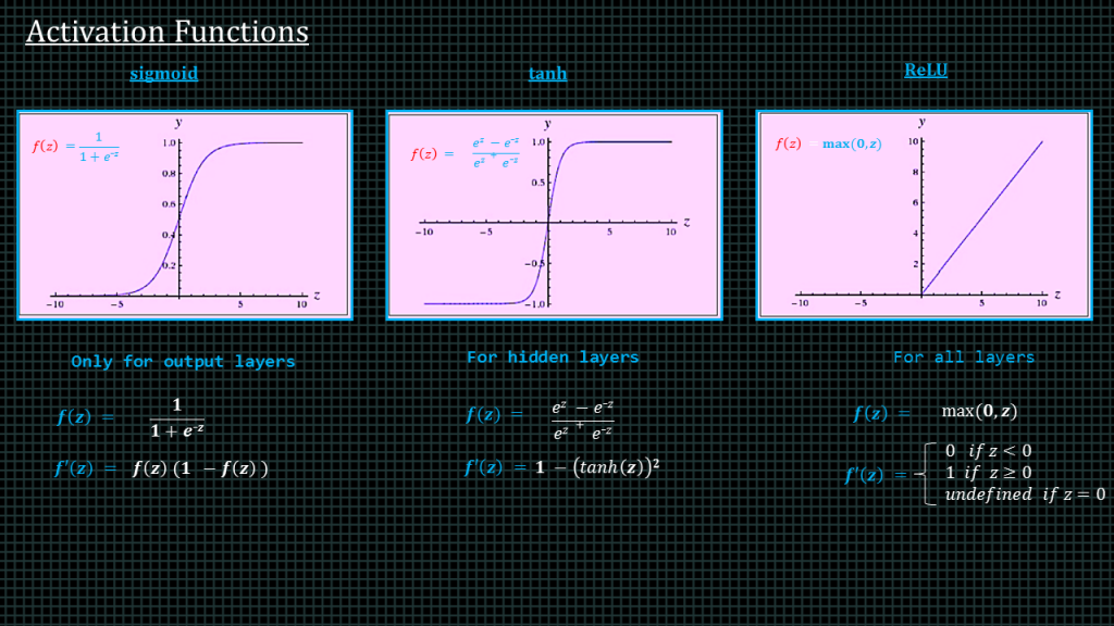
The 3 most popular activation functions are the “sigmoid”, the “tanh” and the rectilinear unit known as “ReLU” for short.
Sigmoid Activation function: It is a activation function of form f(x) = 1 / 1 + exp(-x) . Its Range is between 0 and 1. It is a S — shaped curve.
The “tanh” is expressed as f(x) = 1 — exp(-2x) / 1 + exp(-2x). It’s output is zero centered because its range in between -1 to 1 i.e -1 < output < 1
The “ReLU” is expressed as max(0,x) i.e if x < 0 , R(x) = 0 and if x >= 0 , R(x) = x. It is most popular one among the 3.
The sigmoid function is good for output layers only. The “tanh” performs best when used in hidden layers. The “ReLU” is versatile and good for all layers.
We also show over here the derivatives of these activation functions. We shall implement both the functions and their derivatives in ode later.
Add Comment