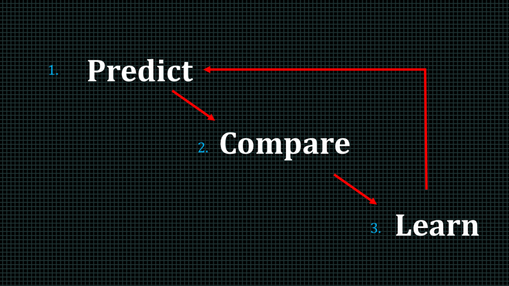
On a high level, the training of a machine learning model typically involves 3 step.
We first predict the result, we compare the predicted result expected resulted, then we learn the difference between the predicted result and the expected once we have learnt the difference we adjust certain parameters of our algorithm in order to reduce the difference between the predicted result and the expected result for next prediction. We are going to spend hours dealing with these 3 steps.
Predict
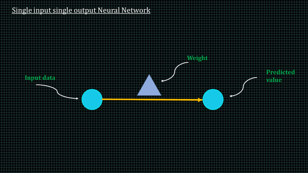
This arrangement over here represents a single input single output neural network.
We have the input, the weight and then the predicted value.
The input interacts with the weight to produce the predicted value.
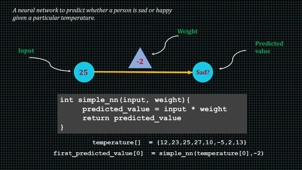
Lets say this is a simple neural network to predict whether a person is sad or happy given a particular temperature.
In this very simplified example we can consider sad and happy to be a numerical value, we could say are number above 10 is considered happy and any number below 10 is considered sad. We shall how to encode words into numerical values later in this course.
If we are to write the pseudo code for this very simplified neural network this is what it will look like. To find the predicted value we simply multiply the input by the weight.
Very simple right. Predicted value = input time weight.
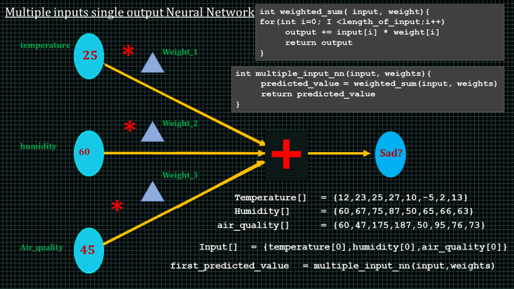
Now lets increase number of inputs to 3.
lets say we want to predict whether a person is sad or happy given the temperature, humidity and air quality.
This is what the neural network will look like. Not that we hve 3 weights, one for temperature, one for humidity the third one for air_quality. To compute the predicted_value,we perform what is called the weight sum.This means we threat this neural network as 3 separate single input, single output neural networks and then add up the predicted values of the 3 separate networks. This is what the pseudocode looks like. We multiply temperature input by weight, we multiply humidity input by weight2, we multiply air quality input by weight 3,and then we add up the 3 products.
Let say we have an array of temperature values.
An array of humidity values and an array of air_quality values.
We perform the first prediction using this pseudo code.
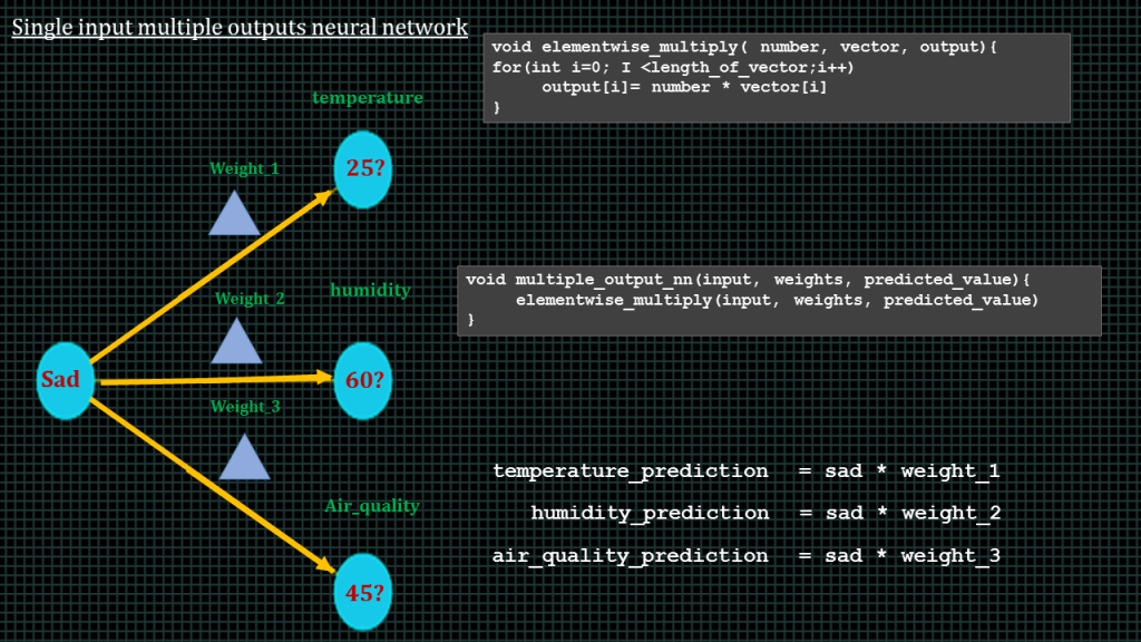
Now lets take a look at a single input multiple ootputs neural network
Lets say we have the mode of a person to be sad and we want to predict the temperature, the humidity and the air_quality.
This is what the network looks like. Can you pause the video and guess how we can compute the predicted values
Ok. To find the temperature_prediction we take the input and multiply it by the temperature weight.
To find the humidity_prediction, we take the input and multiply it by the humidity weight. Likewise to find the air_quality prediction we take the air quality and multiply it by the air quality weight.
This is what the function to perform this type of elementwise multiplication will look like.Over here, number represents the input, since it is a single value for all. Vector represents the array containing the 3 weights, a vector is basics a 1-dimensional array. Output is an array to store the outputs.
This is how we could write the single input multiple output neural network function. Very simple, very straight forward
Now lets take a look at the multiple input multiple output neural network.
The multiple inputs multiple outputs neural network is a combination of the multiple inputs single output neural networks.
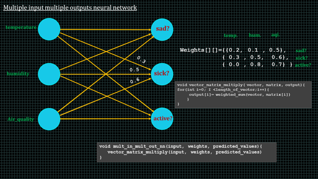
Now lets say, given the temperature, humidity and air quality apart from just predicting whether a person is happy or sad we also when to predict whether they are sick or healthy as well as predict whether they are active or in active.
The simplest way to solve this is to view it as 3 separate multiple inputs single output neural networks.
First we take the inputs of temperature, humidity and air quality, multiply each input with its respective weight, add up the 3 products and then we get the prediction for sad or happy.
We repeat the same to predict sick or healthy
And then repeat it once more to predict active or inactive.
Not that the inputs for predicting the 3 outputs are the same however the weights are different. However a different set of weights is used to predict the 3 outputs.
We can arrange the weights as a 2 dimensional array like this.The first row represents the weight for predicting sad or happy, the second row represents the weight for predicting sick or healthy, and third row represents weights for predicting active or inactive.
The first column in each row represents weights for the temperature input, the second column represents weights for the humidity inputs and the third row represents weights for the a quality input.
To compute the multiple inputs multiple outputs neural network we have to perform a vector matrix multiplication.
Like this function over here, the vector is the 1 dimensional array that contains our inputs and the matrix is the 2 dimensional array that contains the weight.
The pseudo function will compute the 3 predictions of our multiple inputs multiple outputs neural network.
Finally lets examine the neural network with a hidden layer.
The neural network with one hidden layer is a combination of the multiple-inputs single-output and single-input multiple outputs neural network.
Essentially we take the output of one layer and feed it as input of another layer.
Later on in the course you will understand why our neural network will require hidden layers.
Lets see how the prediction of sad can be derived.
We start from the inputs by taking the temperature input multiplying it by its corresponding weight, taking the humidity input multiplying it by its corresponding weight, taking the air quality input multiplying it by its corresponding weight.
We then add the 3 products together, the will give us hidden 0, we then repeat the same sequence to derive hidden 1 and hidden 2.
After we have derived hidden0, hidden1 and hidden3 , we multiply hidden 0, hidden1, hidden3 by their corresponding weights and then we add up the 3 products to get the prediction of sad.
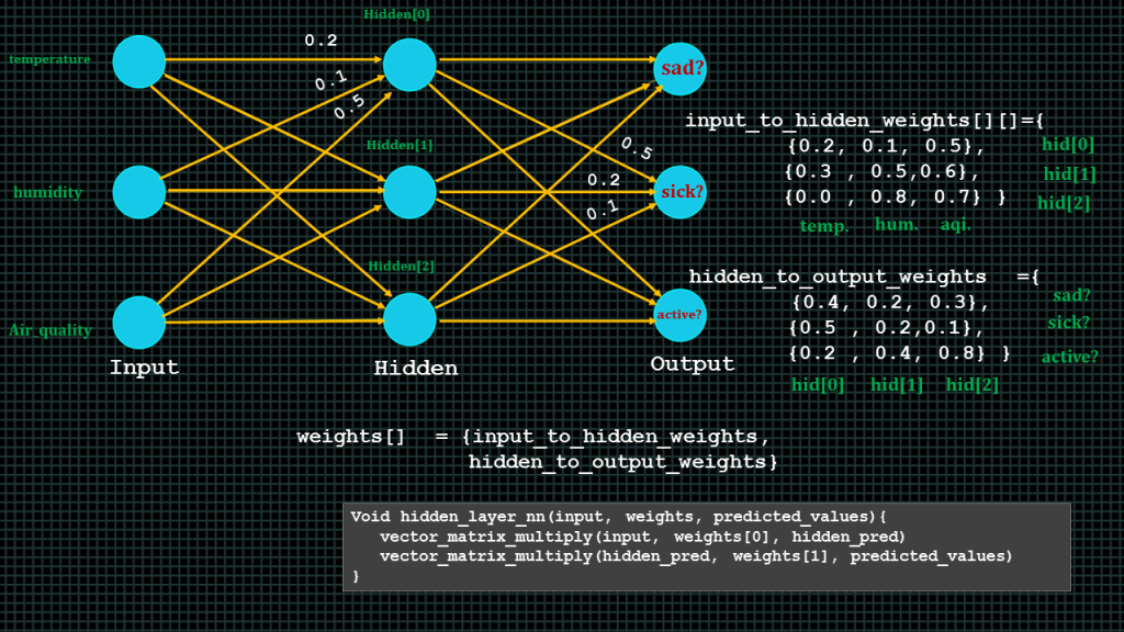
To compute all predictions we will have to perform 2 consecutive vector matrix multiplication.
We will have two sets of weights. The first set will be the weights for the input to hidden layer computation and the second set will be the weight for the hidden layer to output layer computation.
To compute our neural network. We first multiply our vector of inputs by the matrix of input_to_hidden_weights, this shall result in a vector, and like a mentioned earlier a vector is simply one dimensional array. This vector shall contain hidden0 hidden1 and hidden2, we take this vector and multiply it by the hidden to output weights matrix. This vector matrix multiplication shall also result in a vector the vector shall contain the prediction for sad, sick and active.
Compare
Earlier on we mentioned there are generally 3 activities involved in training a machine learning model. Predict, compare and learn.
In the previous lessons we saw how prediction is down. In this lesson we shall how comparison can be made.
Lets take out simple neural network again.
We learned that we predict by multiplying the input by the weight.
Now we are going to introduce another parameter known as error
We find error by subtracting the value we expected from the value we predicted and then squaring the answer.
We square it because we want it to be always positive.
Understanding Data Representation
In this section we shall talk about the basic data types often used in machine lesson.
Tensor is a basic data structure in machine learning.
It is the container of data. This is where tensorflow gets its name.
A tensor of a single number is known as a scaler. For example, the variable x is a scalar.
A tensor of 1 dimension is known as a vector. The example x over here is a 1 dimension tensor and also a 4 dimensional vector because it has 4 elements
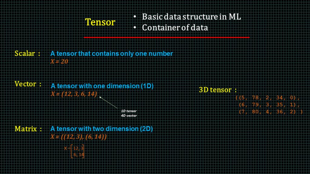
A matrix is a tensor with 2 dimensions.
In other words a 2d array like the example here.
We can have a tensor with an arbitrarily large dimension.
For example this is a 3D tensor.
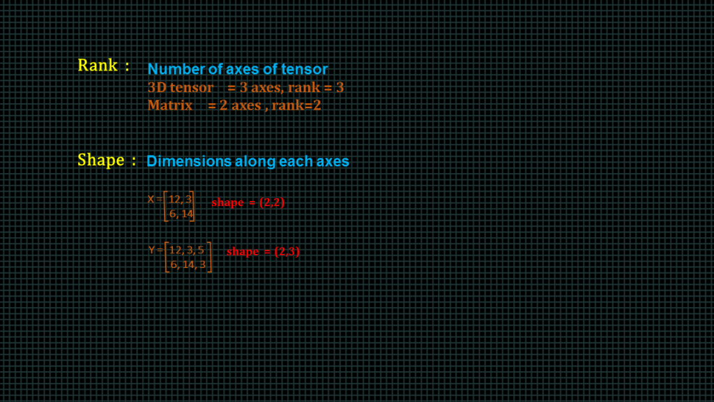
The number of axes of a tensor is known as its rank. The rank of a 3d tensor is 3 and rank of a 2d tensor is 2
The shape of a tensor implies the dimension along each axis of the tensor
X in this example has a shape of 2 by2
Y has a shape of 2 by 3
Learn
Understanding Gradient descent
In this sectionwe are going to talk about the “learning” part of machine learning.
In machine learning when we say learning we simply mean reducing error.
Learning involves calculating the direction and amount by which we need to change the weights in order to reduce the difference between the predicted value and the expected value. Ideally our goal is to make the predicted value as close to the expected value as possible. As we mentioned earlier the difference between the predicted value and the expected value is what we call error. We square this difference to ensure that it always a positive number
We are going to introduce a new variable known as error direction and amount.
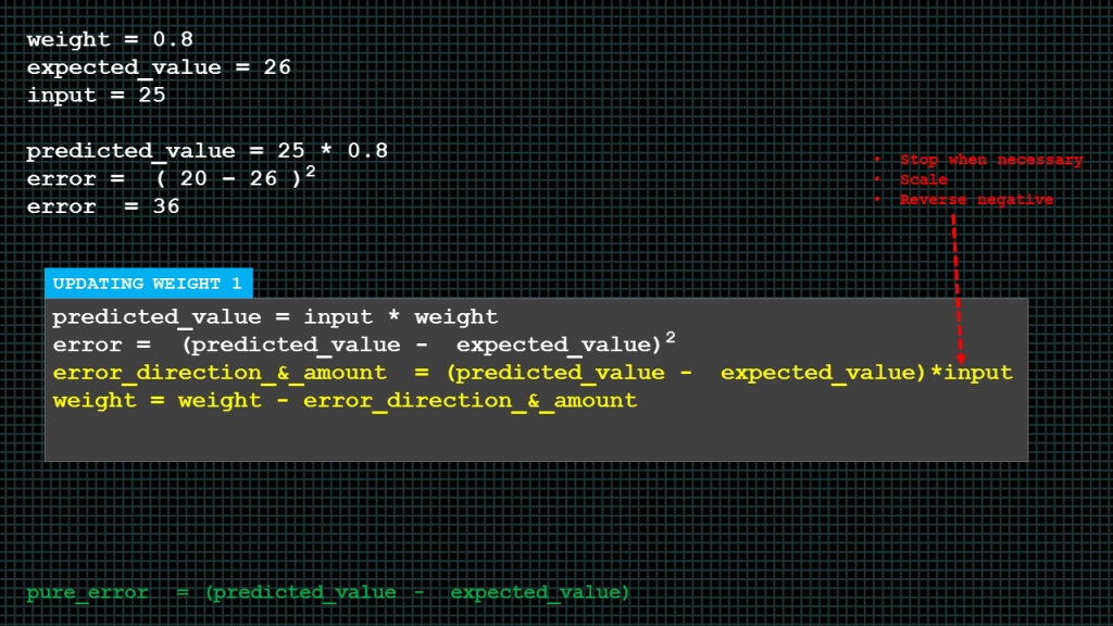
To find the error direction and amount, we subtract the expected value from the predicted value and then we multiply the answer by the input.
We then update the weight by subtracting the error direction and amount from the weight. The answer is the new weight, this new weight is what is multiplied by the input to get the next predicted value.
Predicted value minus expected value is what is known as pure error. Not that over here we do not square the answer.
The pure error tells us the direction and how much we missed, by direction I mean whether positive or negative.
We multiply we multiply by the input to get 3 effects.
If the input is 0 then it will force the error direction and amount variable to be zero because there is nothing to learn.
Multiplying the pure error by input will reverse the sign and direction of the error direction and amount variable in the situation where the input is negative.
If the input is big we want the weight update to big as well and we get this scaling effect also by multiplying the pure error by the input. Because this third effect could get out of hand we will introduce a new constant known as the learning rate, denoted by alpha to prevent the over scaling effect.
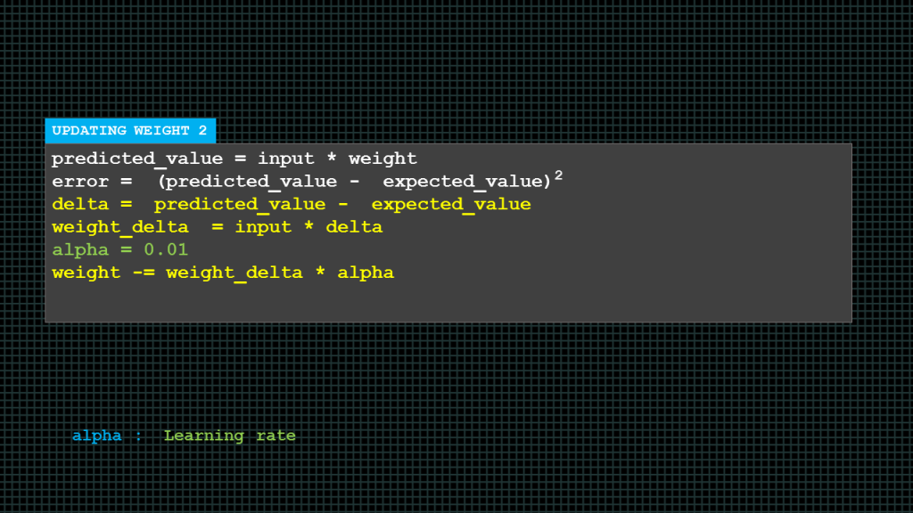
In this pseudocode rather compute the error amount and direction in one line we have broken it into two lines and also introduced 2 new variables known as delta and weight delta.
We find delta by subtracting the expected value from the predicted value.
Weight delta is computed by multiplying delta by the input. In effect weight delta is the same as what we previously had as error direction and amount.
Now, we update the weight by multiplying the weight delta by the constant alpha which is the learning rate. And then subtracting the answer from the current weight the answer because the updated weight value.
Alpha here is set at 0.01.
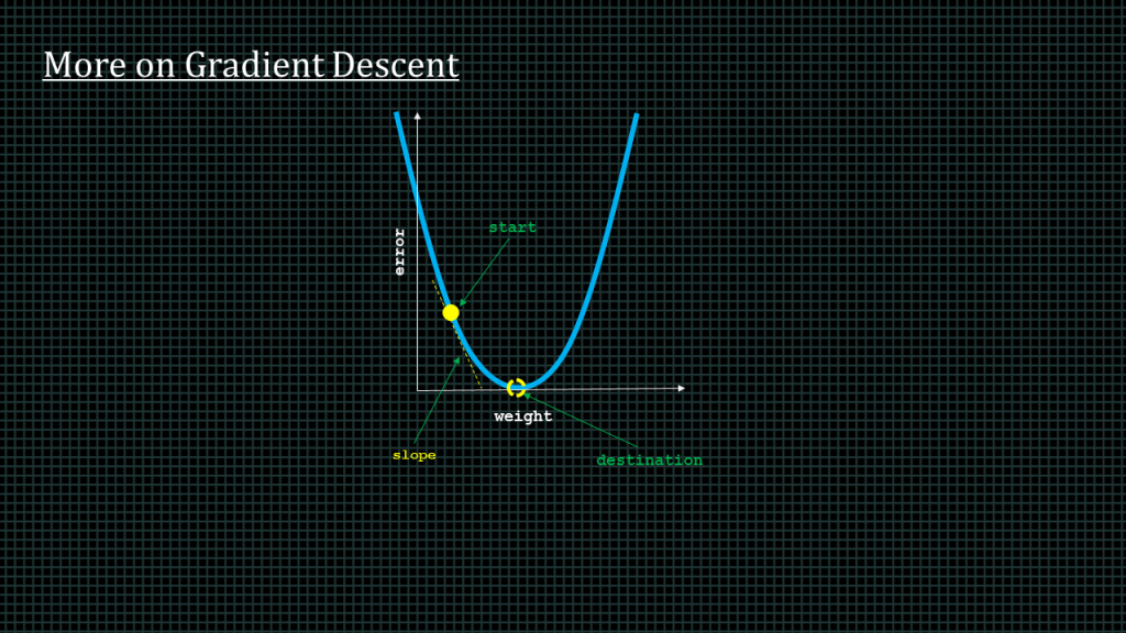
This blue curve here represents every value of error. The yellow dot is the point of both the current weight and error.
The dotted circle is where we want to get to. That is where the error equals zero.
As we can see the slope points to the bottom, because of this no matter where we are on the curve we can use the slope to help the neural network reduce the error.
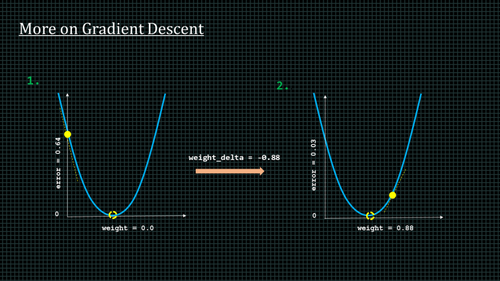
Lets say this is an initial state, with error at 0.64 and weight at 0. Lets say we compute weight delta and get a value of -0.88
When we update the weight with this weight delta value, we get this new plot.
The error reduces the error reduces. As we can see the dot is closer to zero than it used to be. The weight value updates to a value of 0.88. As we can see the dot overshoots our desired destination. We will have to update the weight again until we get as close as possible to our desired destination which is the dashed circle.
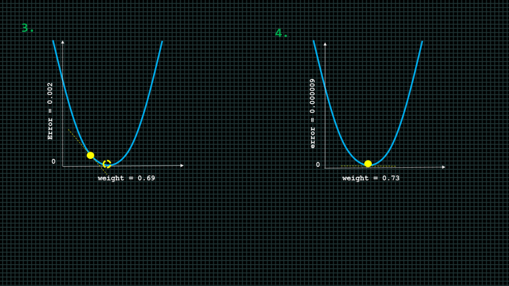
Lets say we update the weight again after a computation of weight delta and its slightly overshoots in the opposite direction but with lesson error than before. This updating of weight continues until we get to the destination as close as possible and the error is as close to zero as possible.

Add Comment